ddPlot(
  x,
  y,
  scale = FALSE,
  location = FALSE,
  name = "X",
  name_y = "Y",
  title = "Depth vs. depth plot",
  depth_params = list()
)

Arguments

x	The first or only data sample for ddPlot.
y	The second data sample. x and y must be of the same space.
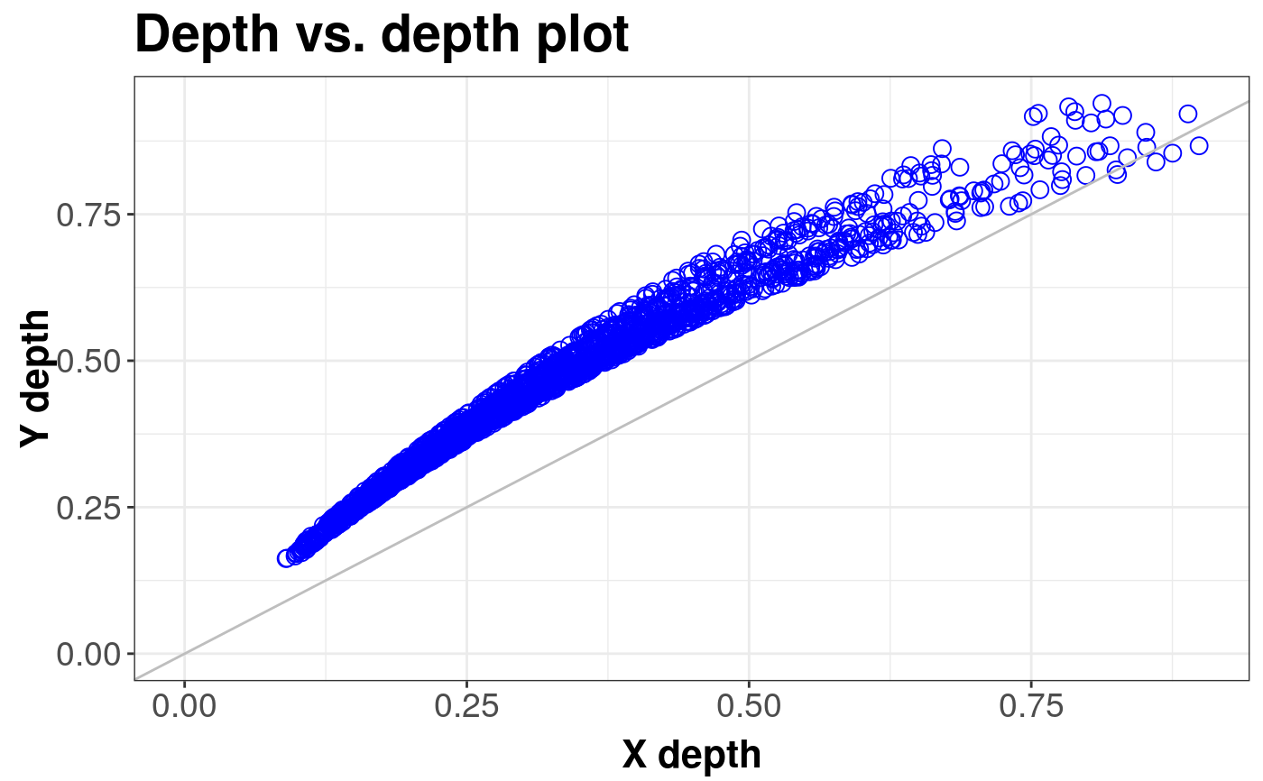
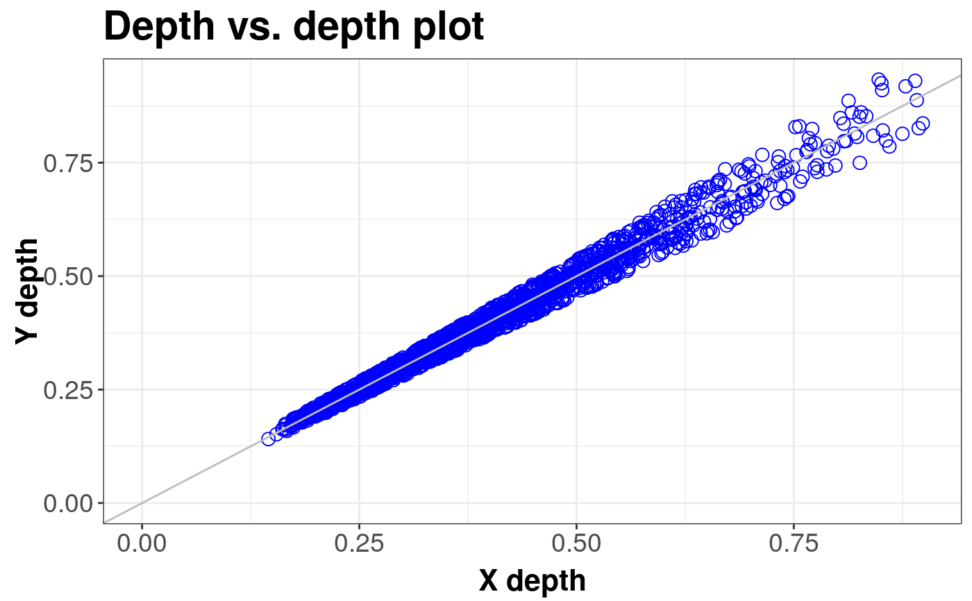
scale	logical. determines whether the dispersion is to be aligned.
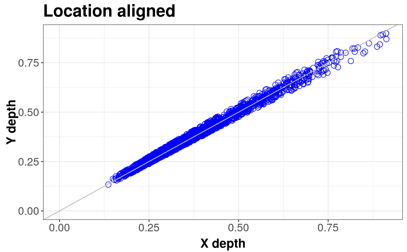
location	determines whether the location is to be aligned to 0 vector with depth median.
name	name for data set x. It will be passed to drawing function.
name_y	as above for y
title	title of the plot.
depth_params	list of parameters for function depth (method, threads, ndir, la, lb, pdim, mean, cov, exact).

Details

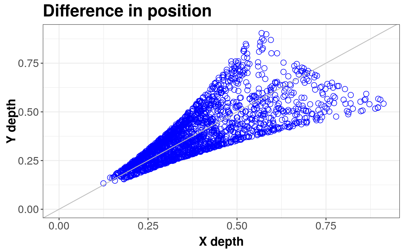
For two probability distributions F and G, both in Rd, we can define depth vs. depth plot being very useful generalization of the one dimensional quantile-quantile plot: DD(F,G)={(D(z,F),D(z,G)),z∈Rd}

Its sample counterpart calculated for two samples Xn={X1,...,Xn} from F, and Ym={Y1,...,Ym} from G is defined as DD(Fn,Gm)={(D(z,Fn),D(z,Gm)),z∈{Xn∪Ym}}

References

Liu, R.Y., Parelius, J.M. and Singh, K. (1999), Multivariate analysis by data depth: Descriptive statistics, graphics and inference (with discussion), Ann. Statist., 27, 822--831.

Liu, R.Y., Singh K. (1993), A Quality Index Based on Data Depth and Multivariate Rank Test, Journal of the American Statistical Association vol. 88.

Examples

library(sn)
library(mvtnorm)

# EXAMPLE 1: Location difference
standard <- mvrnorm(1000, c(0, 0), diag(2))
shift <- mvrnorm(1000, c(0.5, 0), diag(2))
ddPlot(x = standard, y = shift, title = "Difference in position")
#> DDPlot
#> 
#> Depth Metohod:
#> 	 Projection
ddPlot(x = standard, y = shift, location = TRUE, title = "Location aligned")
#> DDPlot
#> 
#> Depth Metohod:
#> 	 Projection

# EXAMPLE 2: Scale difference
standard <- mvrnorm(1000, c(0, 0), diag(2))
scale <- mvrnorm(1000, c(0, 0), 4 * diag(2))
ddPlot(x = standard, y = scale)
#> DDPlot
#> 
#> Depth Metohod:
#> 	 Projection
ddPlot(x = standard, y = scale, scale = TRUE)
#> DDPlot
#> 
#> Depth Metohod:
#> 	 Projection